2019-12-24: Christmas Songs

This week’s #TidyTuesday challenge examines Christmas songs appearing on the Billboard Top 100 from the 1950s to the 2010s.

See the full details here

This week’s data is about Christmas songs on the hot-100 list! Clean data comes from Kaggle and originally from data.world. The lyrics come courtest of Josiah Parry’s genius R package. It has several useful functions, mainly built around grabbing lyrics for specific artists, songs, or albums. Data source here

Step 1: Data Prep

I decided to focus on word frequencies within all songs that ever occurred on the Billboard Top 100. Since I still wanted to maintain a record of both the number of occurrences, as well as the overall sentiment, I aggregated the original dataset and summarized the number of occurences over the past 60+ years.

For whatever reason, the original dataset did not contain the lyrics for each song. I figured this was a great time to take advantage of the Genius package. If you’re interested, check out the arduous process of collecting lyrics to such hits as “What Can You Get a Wookie For Christmas (When He Already Owns a Comb?)” in my source code here

Step 2: Tokenize Lyrics, Prep for Sentiment Analysis

DETAILS ON CHOOSING BING VS.

# set lexicon
bing <- get_sentiments("bing")
lyrics<-agg%>%
  select(-1:-4)%>%
  select(-sentiment)
lyrics$lyrics<-as.character(lyrics$lyrics)
bing$sentiment<-as.character(bing$sentiment)

Step 3: Conduct Sentiment Analysis

# counting negative / positive words
sentiment <-lyrics%>%
  unnest_tokens(word, lyrics) %>% 
  anti_join(stop_words) %>%
  # join afinn score
  inner_join(bing) %>%
  count(word, sentiment, sort = TRUE) %>%
  ungroup() %>%
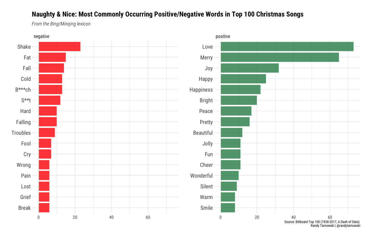
  filter(word!="bum")

Step 4: Visualization

# FINAL PLOT
sentiment %>%
  group_by(sentiment) %>%
  top_n(15) %>%
  ungroup() %>%
  mutate(word = reorder(word, n)) %>%
  ggplot(aes(word, n, fill = sentiment)) +
  geom_col(alpha = 0.8, show.legend = FALSE,  colour="white", stat="identity") +
  facet_wrap(~sentiment, scales = "free_y") +
  labs(y = "Source: Billboard Top 100 (1958-2017, A Dash of Data) \n Randy Tarnowski | @randytarnowski",
       x = NULL,
       title="Naughty & Nice: Most Commonly Occurring Positive/Negative Words in Top 100 Christmas Songs",
       subtitle = "From the Bing/Minqing lexicon") +
  coord_flip() +
  theme_ipsum_rc() + 
  scale_fill_manual(values = c("red", "seagreen")) + 
  theme(axis.text.y=element_text(size=rel(1.25))) +
  theme(plot.subtitle = element_text(face = "italic"))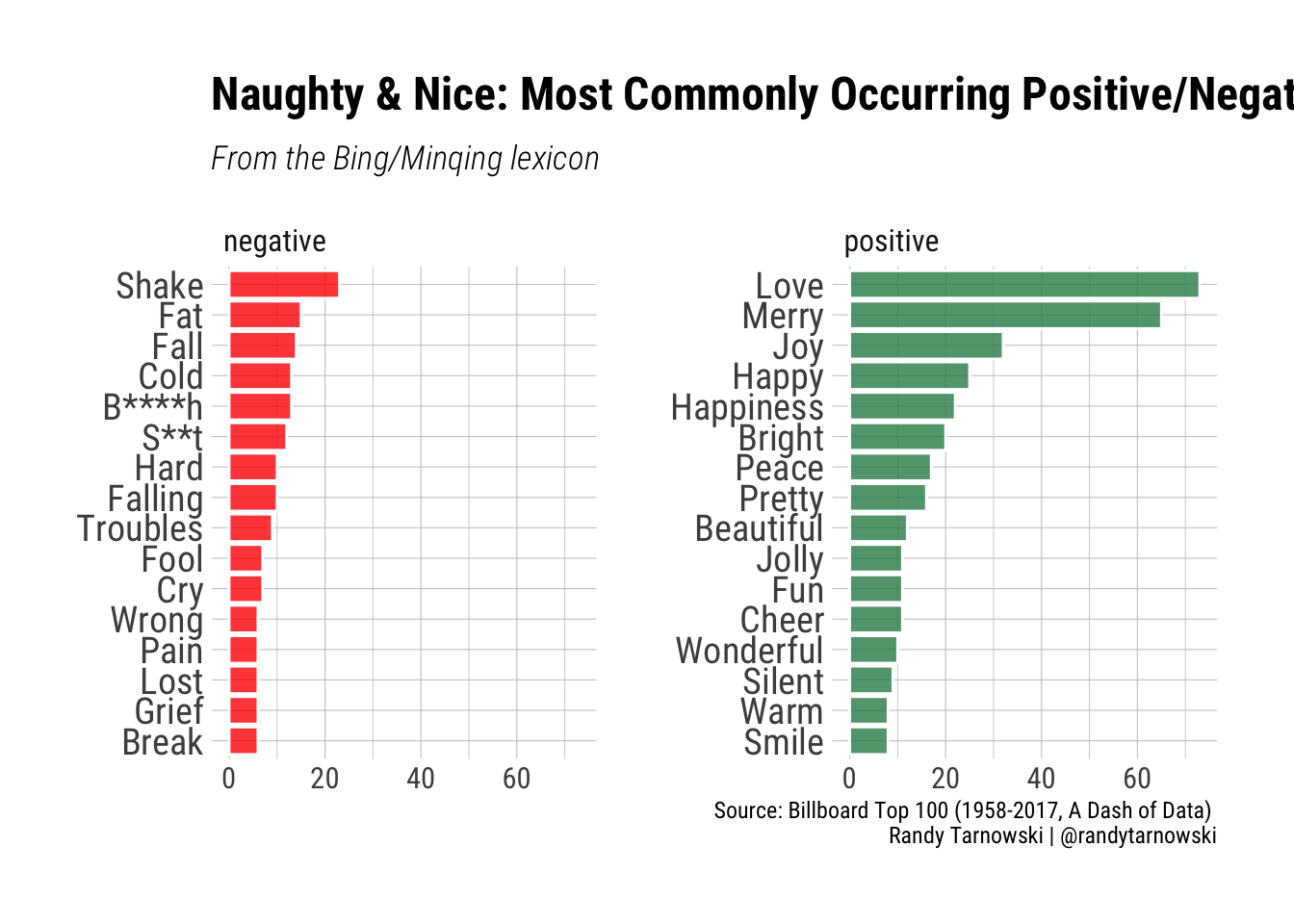

Step 5: Further Analysis

Now that all the lyrics are collected, there are many areas for further analysis. This includes:

• Decade-based Research: Is there a difference in the overall mood of Christmas songs by decade? I’ve always loved the melancholic underpinning of a lot of Christmas songs (e.g., Charlie Brown X-Mas songs, Last Christmas, etc.).
• Alternative Sentiments:

# basic scatterplot
agg<-agg%>%
  mutate(colors=ifelse(sentiment<0, "Negative", "Positive"))

ggplotly(ggplot(agg, aes(x=n, y=sentiment, label=agg$songid, group=colors)) + 
  geom_jitter(width = 10, aes(color=as.factor(colors))) +
  theme_ipsum() + 
    labs(y = "Sentiment (+ is positive, - is negative)",
       x = "Number of Occurences on Top 100",
       title="Sentiment by Number of Occurences on Billboard"))